Background
In minesweeper, to calculate the probability that given square is a mine was proved to be #P-complete. I offer an exponential, heuristically improved approach to finding such probabilities.
How Mine Probability is Defined
Mine probability for a square X is defined as:
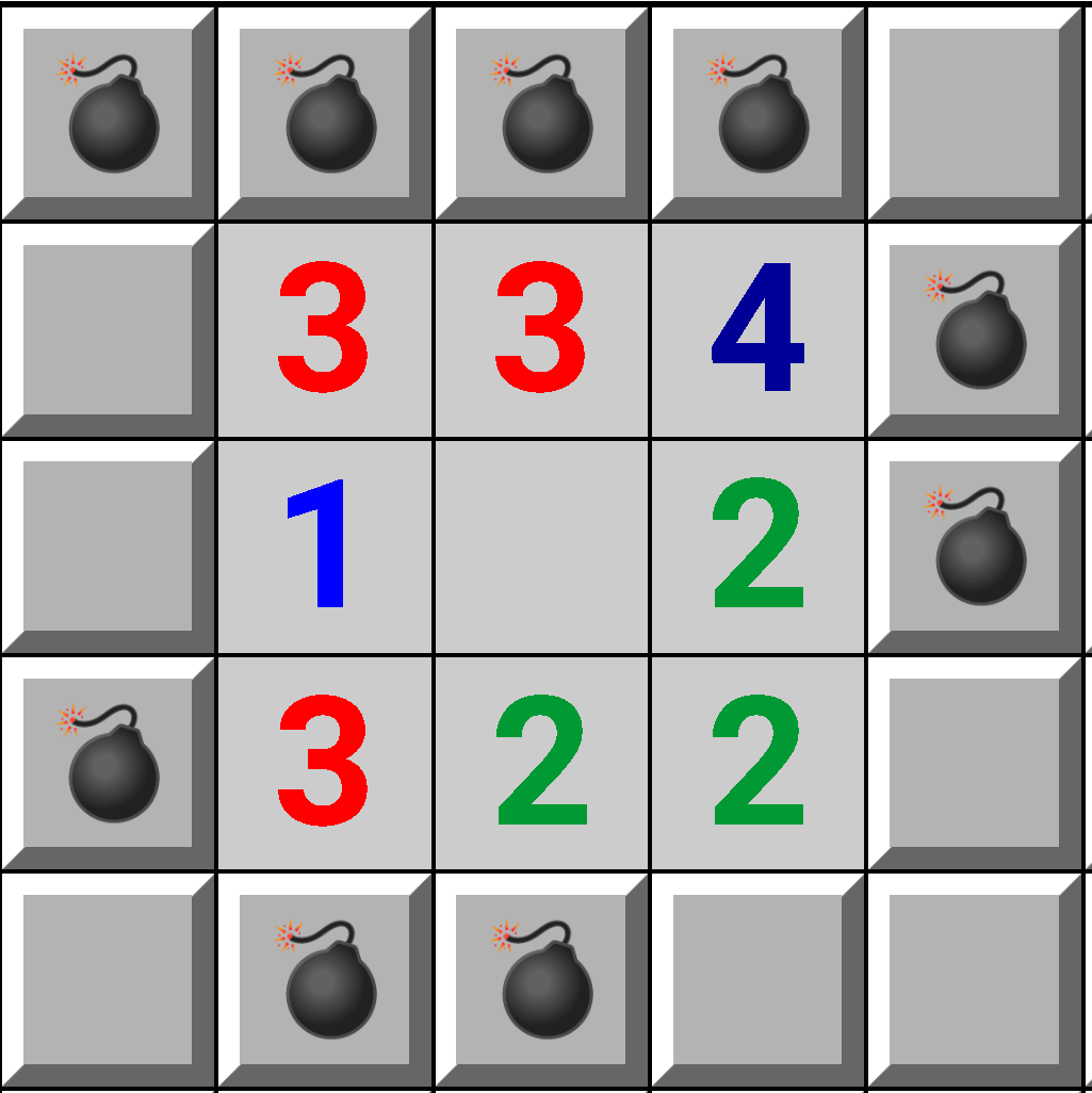
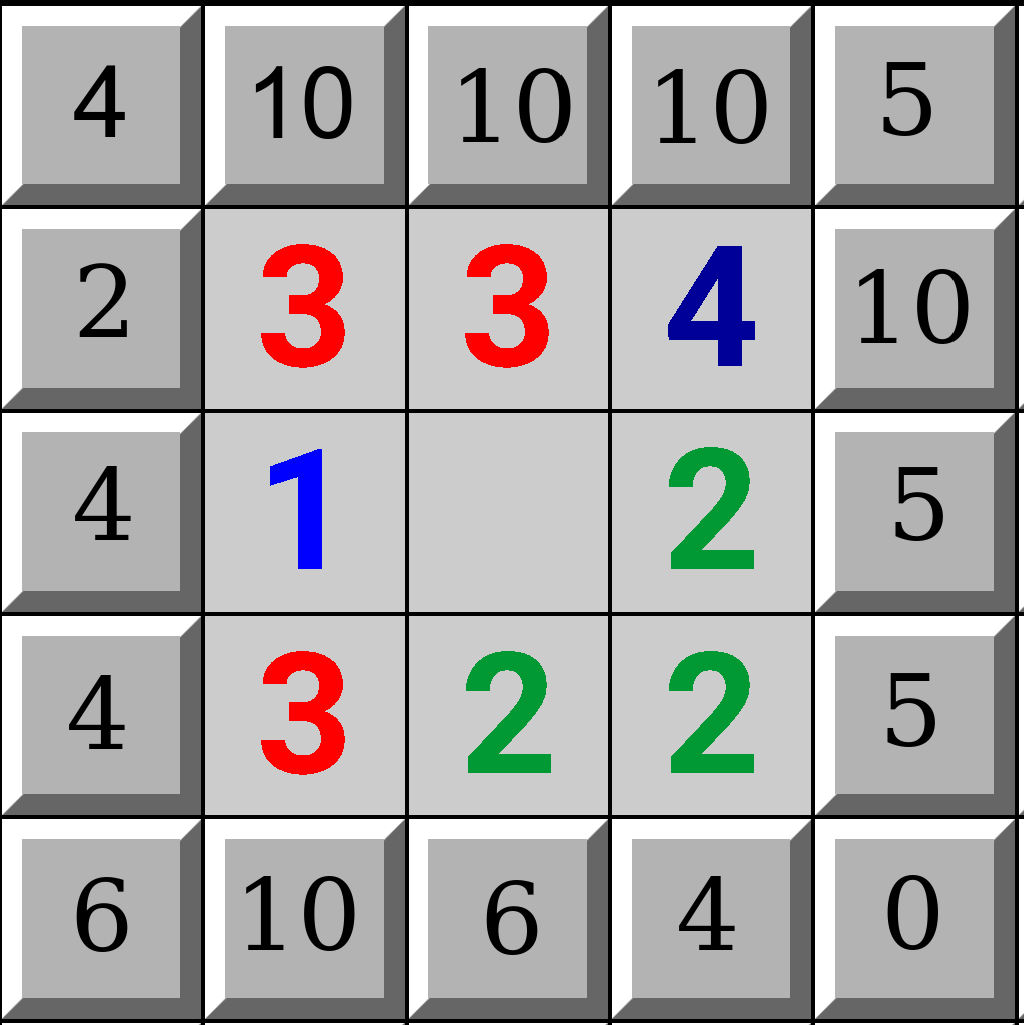
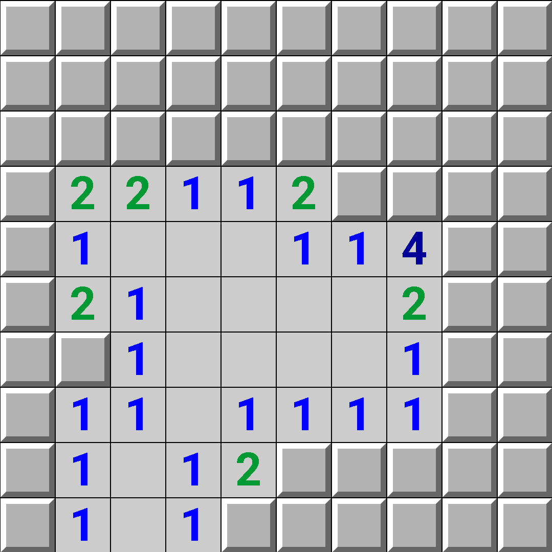
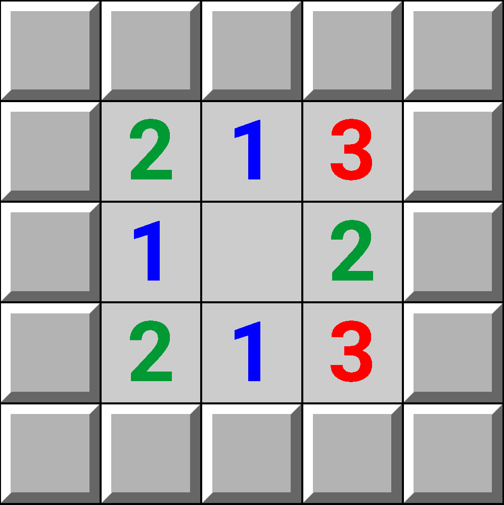
\[\frac{\text{number of mine configurations where X is a mine}}{\text{total number of mine configurations}}\]as each mine configuration has an equal chance of occurring. Let's look at an example board with 20 mines:
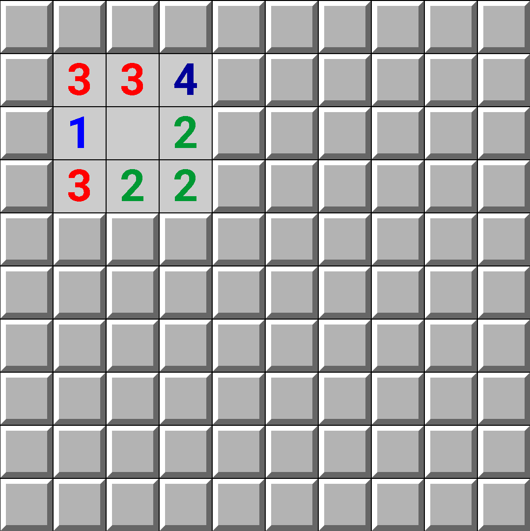
The above board has 10 equally likely configurations of mines:
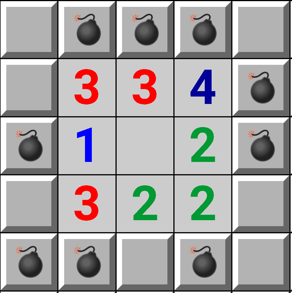
All the configurations have the following in common:
- The red squares are the squares where every configuration has a mine
- The green square had no mine in any configuration
In a sense, it is possible "to deduce" that the red squares are mines, and the green square isn't a mine. For example, the top 3 red squares on the first row are all mines since the middle 3 has only 3 surrounding squares. Thus all three squares must have a mine.
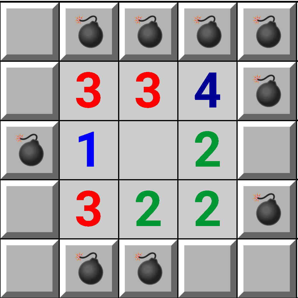
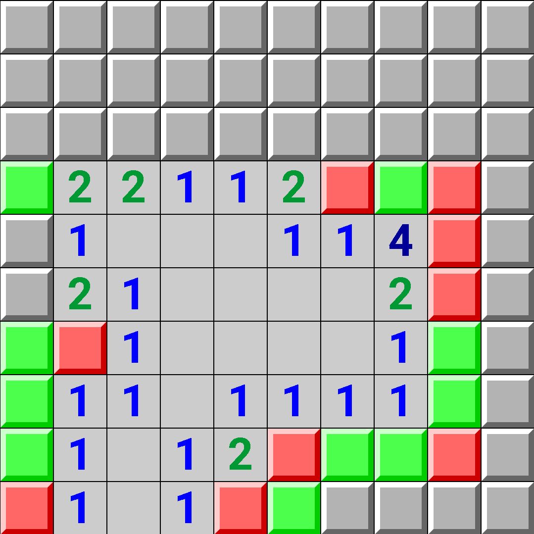
Now what about calculating mine probabilities? For each square, let's count up how many out of the above 10 configurations have a mine:
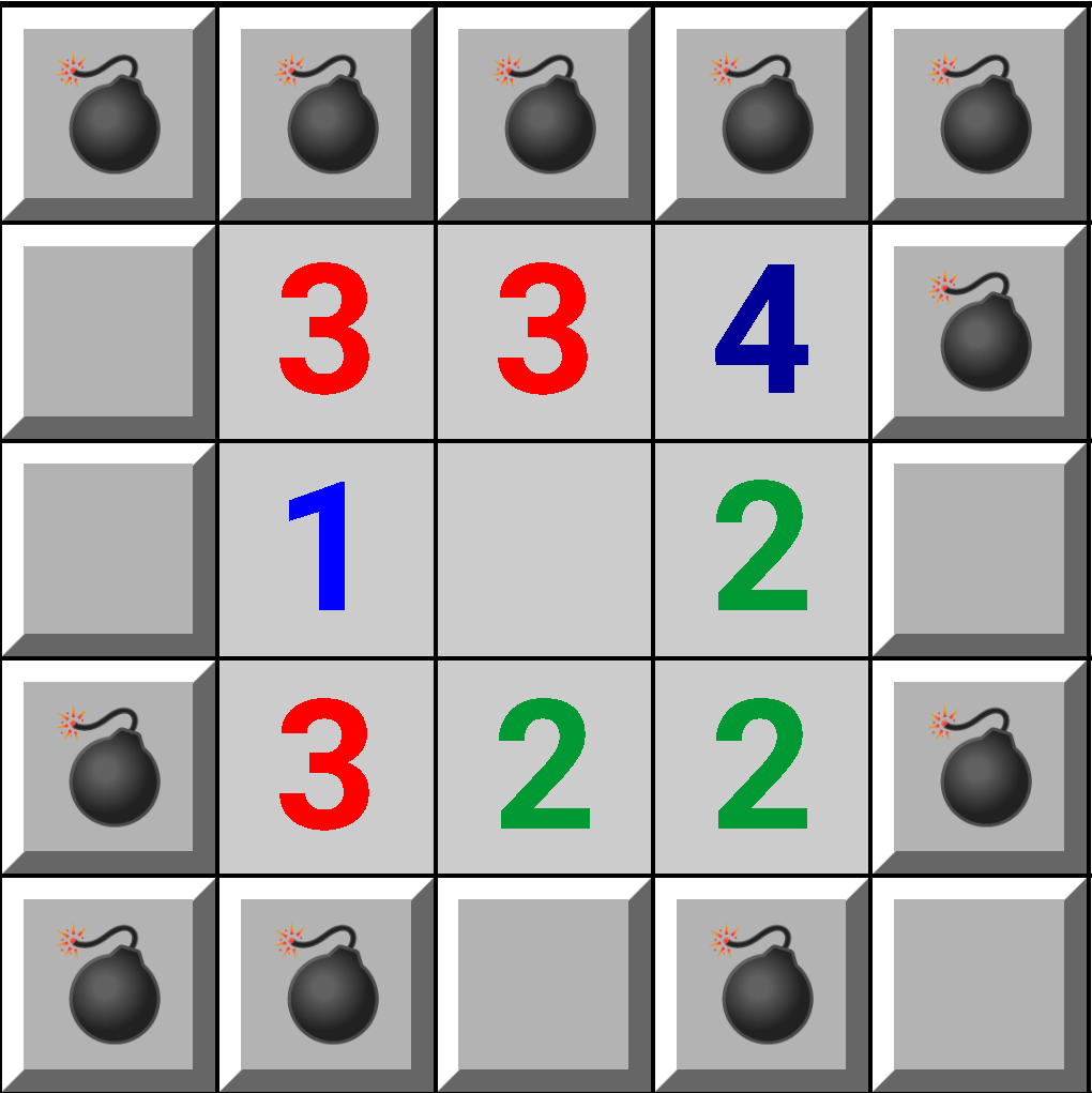
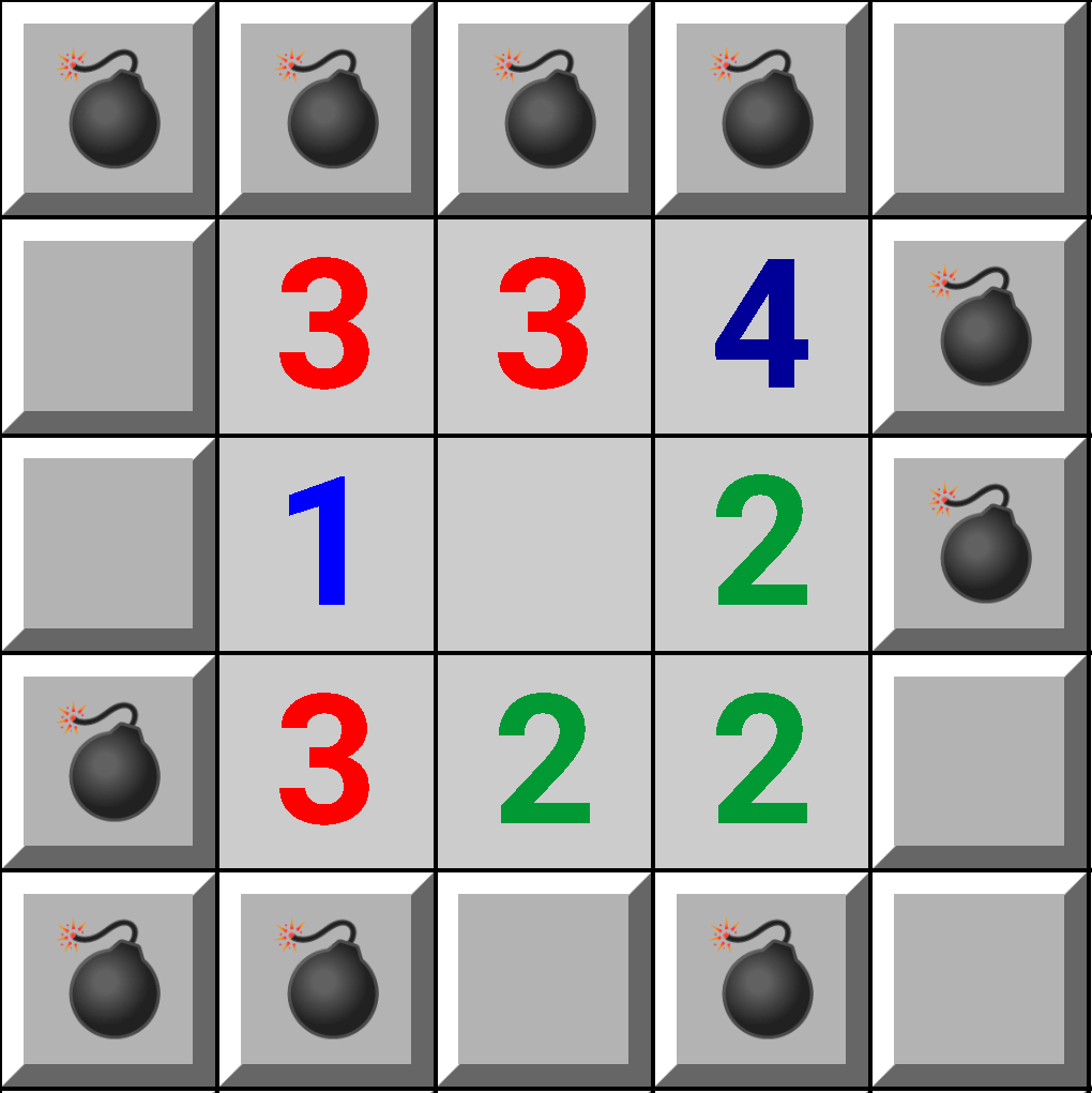
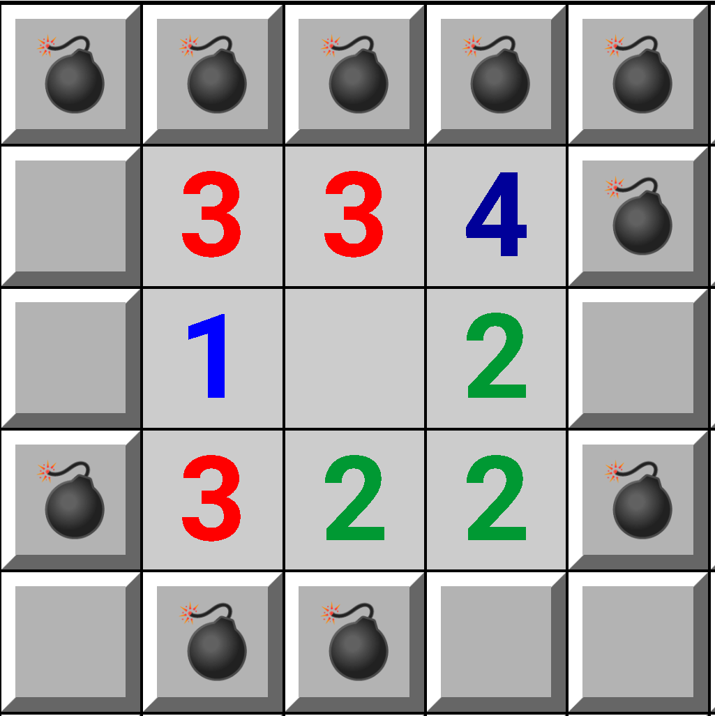
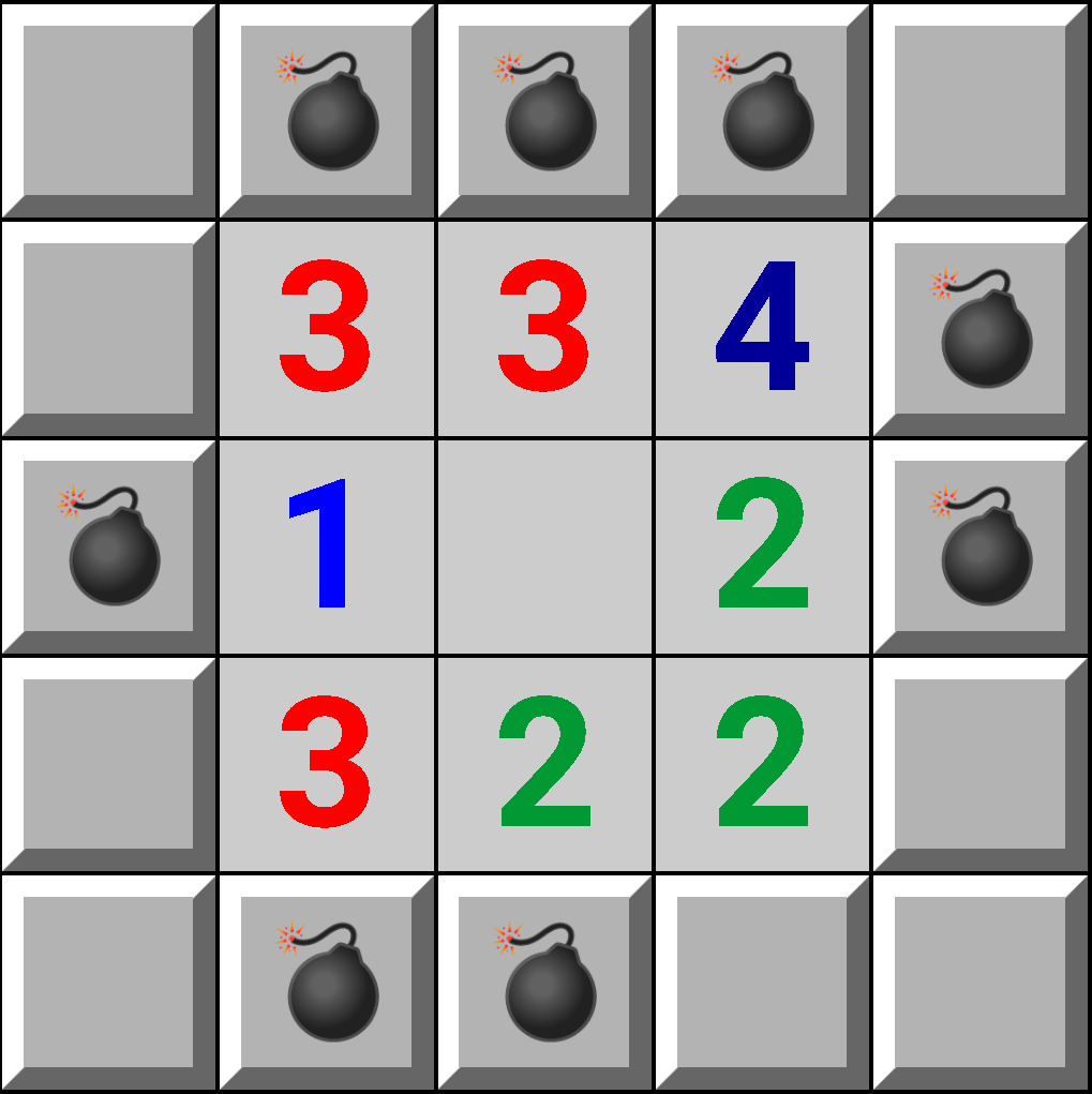
It seems like the top-left square has probability \(\frac{4}{10}\) of being a mine since 4 out of 10 configurations have a mine there. As pointed out in this comment, this is incorrect; it turns out to be more complicated. Let's zoom out to see the entire board again.
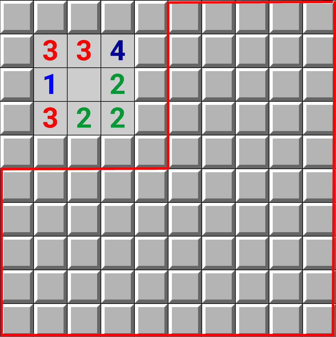
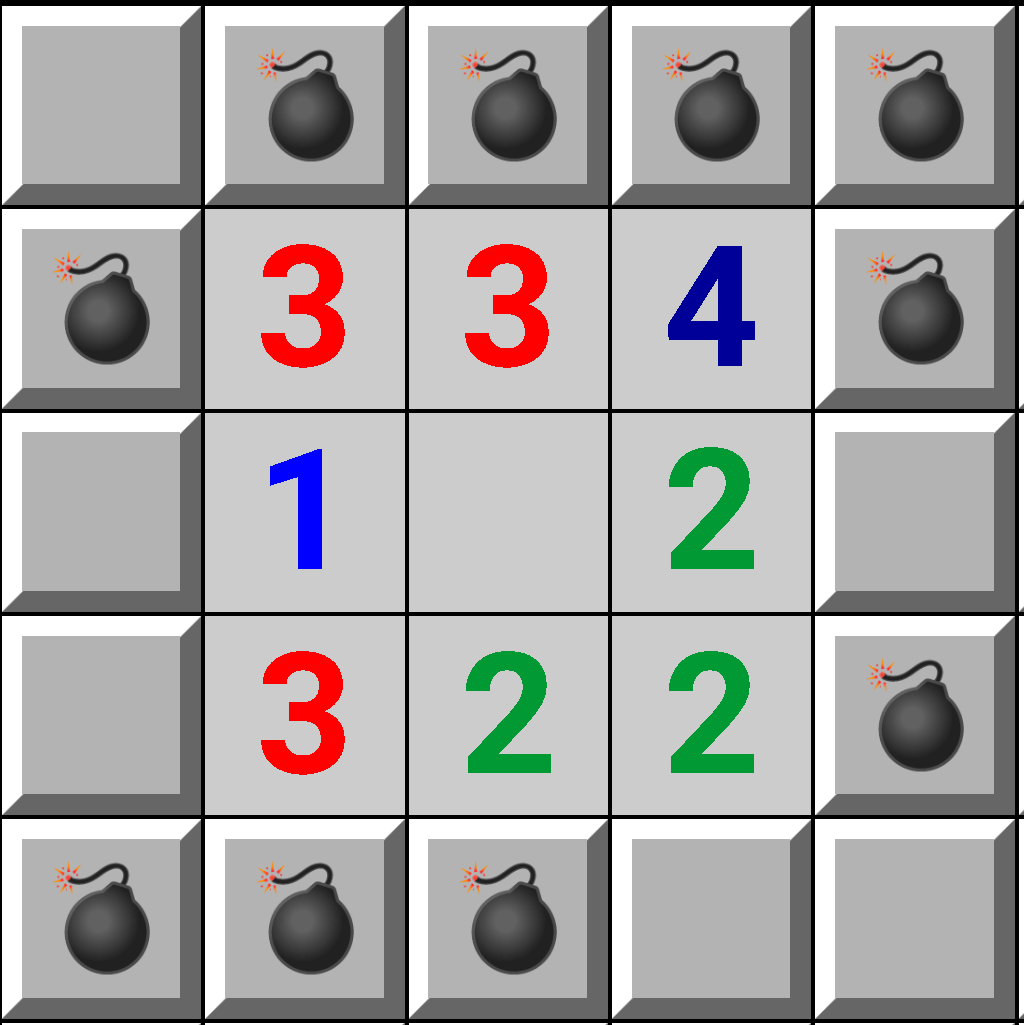
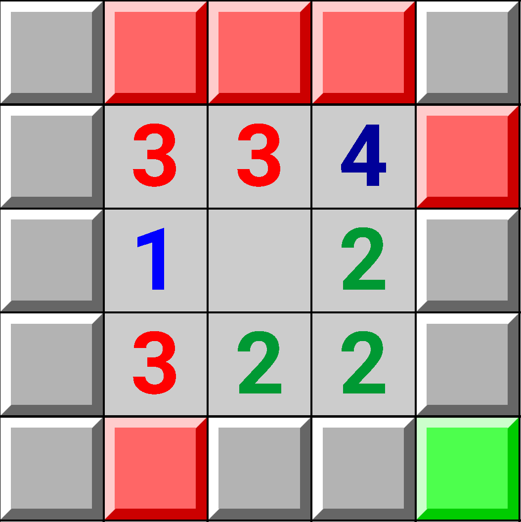
There are 75 squares which weren't accounted for previously
(surrounded in red). Not all configurations of mines have the
same number of mines, and thus aren't weighted equally. For
example
has 8 mines, while
has 11 mines. Recall
there are 20 total mines. We have to choose where to place the
remaining mines among the 75 remaining squares. For example,
since
has 8 mines, we need to
choose \(20 - 8\) squares out of the remaining 75 squares to
place the remaining mines. The number of ways to do this is
\(\binom{75}{20-8} = 26123889412400\). You can think of
\(\binom{75}{20-8}\) as
's "weight". Then, the fraction of "weighted" sums will give the
correct mine probability for each square.
| Number of Mines | Number of Configurations with top-left a mine | Number of Configurations |
|---|---|---|
| 8 | 0 | 1 |
| 9 | 1 | 4 |
| 10 | 2 | 4 |
| 11 | 1 | 1 |
For example, the top-left square has probability: \[\frac{0\binom{75}{20-8} + 1\binom{75}{20-9} + 2\binom{75}{20-10} + 1\binom{75}{20-11}}{1\binom{75}{20-8} + 4\binom{75}{20-9} + 4\binom{75}{20-10} + 1\binom{75}{20-11}} = \frac{14}{103} \neq \frac{4}{10}\] of being a mine.
Let's now define mine probability in general.
- Let \(C\) denote the set of all mine configurations
- Define \(f \colon C \to \{true,false\}\) as follows: \( f(c)=\begin{cases} true & \text{c has a mine in square X} \\ false & \text{c has no mine in square X} \end{cases} \)
- Let \(Y\) denote the number of squares not next to any number, clue. (in the above example, \(Y=75\))
- Let \(M\) denote the total number of mines. (in the above example, \(M=20\))
- Define \(\#m \colon C \to \mathbb{Z}^+\) as follows: \(\#m\left(c\right) =\) the number of mines in configuration c. (in the above example, \(8 \leq \#m(c) \leq 11\))
Then square X has a mine with probability: \[\frac{\sum\limits_{c \in C \mid f(c)} \binom{Y}{M-\#m(c)}}{\sum\limits_{d \in C} \binom{Y}{M-\#m(d)}}.\]
How about squares not next to any number (e.g. the \(Y = 75\) squares)? For these squares, mine probability is: \[\frac{\sum\limits_{c \in C} \frac{M-\#m(c)}{Y}\binom{Y}{M-\#m(c)}}{\sum\limits_{d \in C} \binom{Y}{M-\#m(d)}}.\]
For a given configuration c, \(\frac{M-\#m(c)}{Y}\) is the probability that any of the \(Y\) squares are a mine. And the final probability is a weighted average, where the weight is \(\binom{Y}{M-\#m(c)}\).
Notice the numerator and denominator are huge (in magnitude). For the above example: \[\text{numerator} = 0\binom{75}{20-8} + 1\binom{75}{20-9} + 2\binom{75}{20-10} + 1\binom{75}{20-11}\] \[= 6,681,687,099,710\] but the end result is relatively small (in magnitude): \(\frac{14}{103}\). The reason why most factors cancel is because \[\frac{\sum\limits_{c \in C \mid f(c)} \binom{Y}{M-\#m(c)}}{\sum\limits_{d \in C} \binom{Y}{M-\#m(d)}}= \sum\limits_{c \in C \mid f(c)} \frac{\binom{Y}{M-\#m(c)}}{\sum\limits_{d \in C} \binom{Y}{M-\#m(d)}}= \sum\limits_{c \in C \mid f(c)} \frac{1}{\frac{\sum\limits_{d \in C} \binom{Y}{M-\#m(d)}}{\binom{Y}{M-\#m(c)}}}=\]\[ \sum\limits_{c \in C \mid f(c)} \frac{1}{\sum\limits_{d \in C} \frac{\binom{Y}{M-\#m(d)}}{\binom{Y}{M-\#m(c)}}},\] and \[\frac{\binom{Y}{M-\#m(d)}}{\binom{Y}{M-\#m(c)}}=\frac{\left(M-\#m(c)\right)!\left(Y-M+\#m(c)\right)!}{\left(M-\#m(d)\right)!\left(Y-M+\#m(d)\right)!}.\] Notice \(\left|\#m(c)-\#m(d)\right|\) is small, \(\leq 3\) in most cases, thus most factors in \(\frac{\left(M-\#m(c)\right)!}{\left(M-\#m(d)\right)!}\), and \(\frac{\left(Y-M+\#m(c)\right)!}{\left(Y-M+\#m(d)\right)!}\) cancel.
We can employ one of the following formulas (or their reciprocals):
- \(\frac{\binom{n}{k}}{\binom{n}{k}}=1\)
- \(\frac{\binom{n}{k}}{\binom{n}{k+1}}=\frac{k+1}{n-k}\)
- \(\frac{\binom{n}{k}}{\binom{n}{k+2}}=\frac{\left(k+1\right)\left(k+2\right)}{\left(n-k\right)\left(n-k-1\right)}\)
- \(\frac{\binom{n}{k}}{\binom{n}{k+m}}= \frac{(k+1)(k+2)\dots(k+m)}{(n-k)(n-k-1)\dots(n-k-(m-1))}\)
Implementing Mine Probability
In order to calculate the probability that square X is a mine, we need to calculate 2 things:
- For each square X, the number of mine configurations which have \(m\) mines where X is a mine, (\(0 \leq m \leq M\))
- number of total mine configurations with \(m\) mines, (\(0 \leq m \leq M\))
To calculate these, we employ backtracking:
Even with pruning, this algorithm runs in \(\mathcal{O}\left(\left|squares\right| \cdot 2^{\left|squares\right|}\right)\). The \(\left|squares\right|\) factor comes from handling the base case, and there are at most \(2^{\left|squares\right|}\) base cases (mine configurations). The next section will discuss ways to make \(\left|squares\right|\) smaller.
Splitting by Components
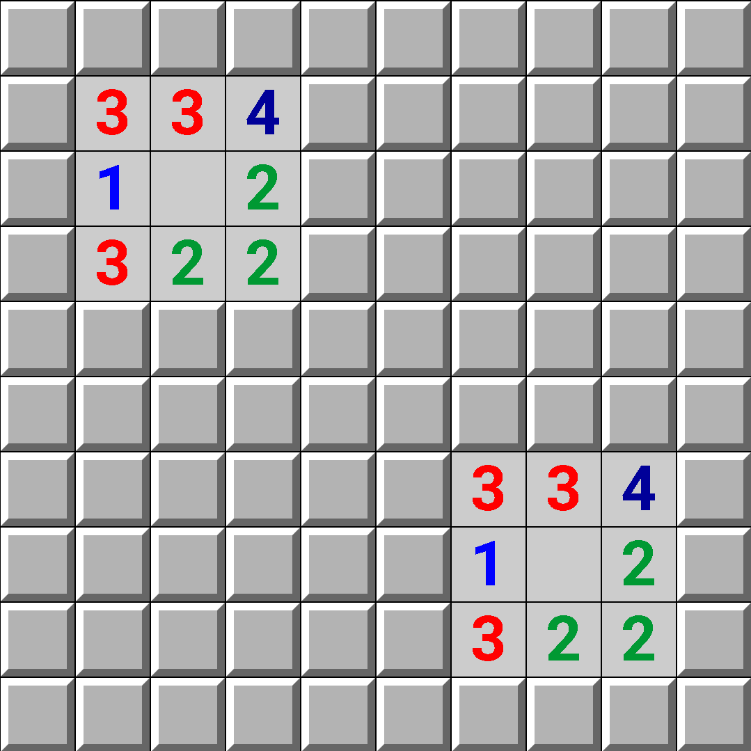
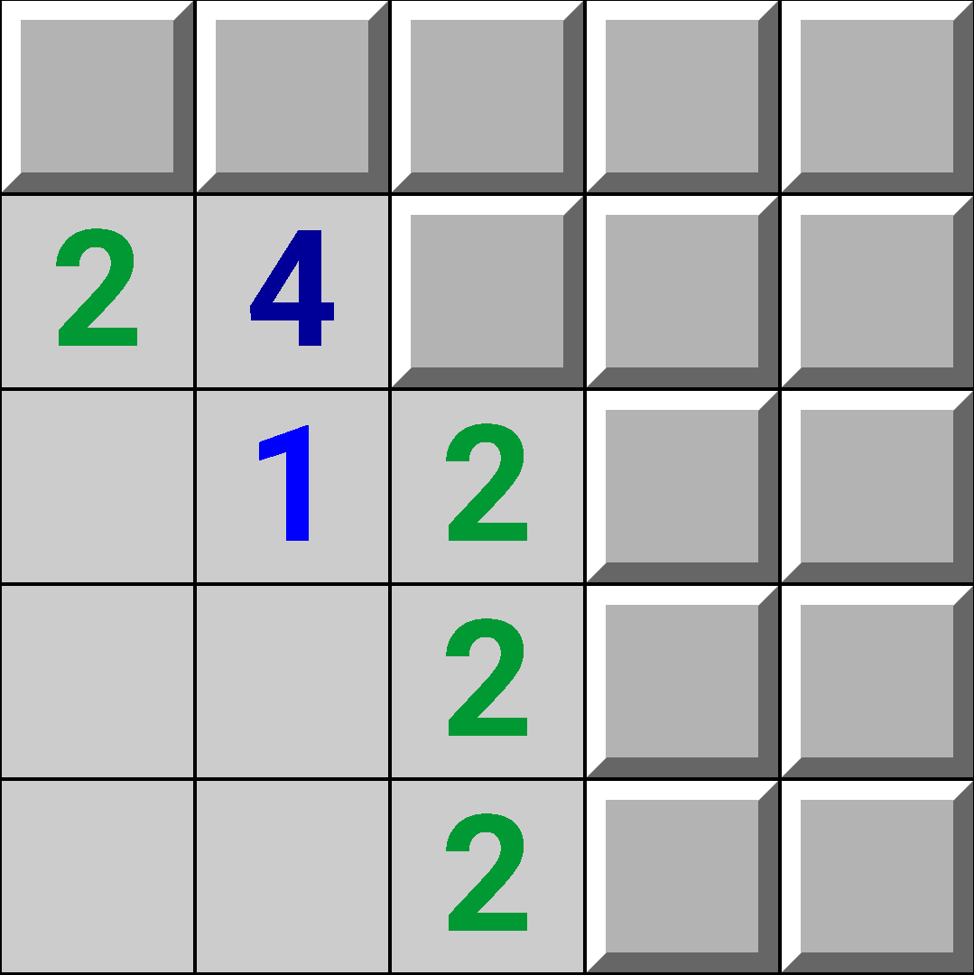
The first optimization, splitting by components, is discussed in other blogs for example this blog. Consider the following board:
Running the backtracking will take roughly \(\left(3+4+11\right)\cdot2^{3+4+11}=4,718,592\) steps. Instead, how about running the backtracking independently on the red, blue, and green components. This will take roughly \(3\cdot2^3+4\cdot2^4+11\cdot2^{11}=22,616\) steps (much smaller).
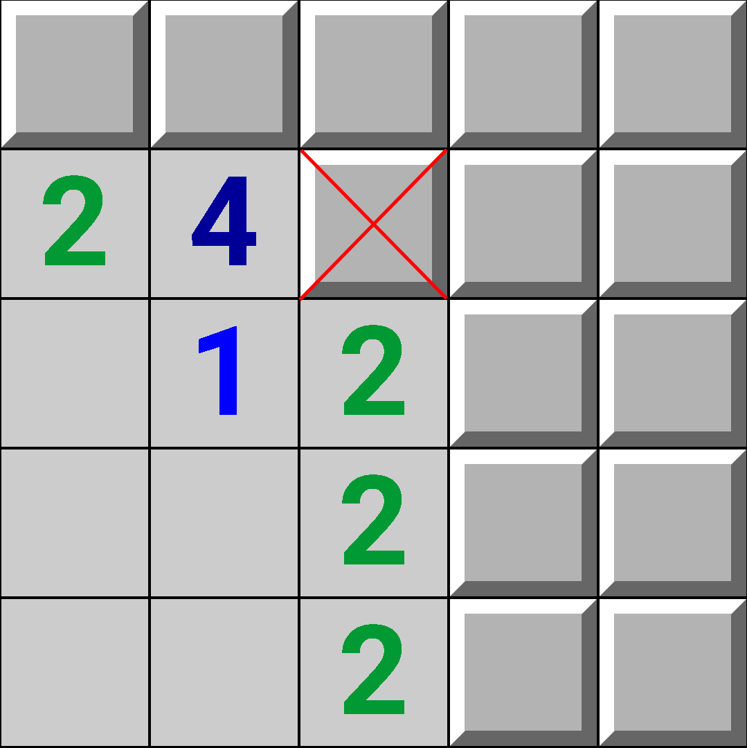
But splitting the backtracking into multiple components makes things difficult. Let's look at another example (there are still 20 total mines):
Both components are the same as earlier, and both can have either 8, 9, 10, or 11 mines. But since there are 20 total mines, if one component has 11 mines, then the other component can only have 8 or 9 mines. In general, the total number of mines has to be in the range \([M-Y,M]\), with \(M,Y\) defined earlier. This leads to the following problem.
You are given \(n\), the number of components (labeled 1, 2, ..., n), and an array \(\#configs[][]\), where
\(\#configs[i][j]\) = number of configurations of mines for the \(i\)-th component which have \(j\) mines, \((1 \leq i \leq n,\;0 \leq j \leq M)\).
Find \(\#totalConfigs[]\) defined as:
\(\#totalConfigs[i]\) = number of configurations of mines which have \(i\) mines when including all components, \((0 \leq i \leq M)\).
This problem is similar to 0-1 knapsack. It's solved by dynamic programming. Let
\(dp[i][j]\) = number of configurations including only components \(1, 2, ..., i\) which have \(j\) mines, \((1 \leq i \leq n,\;0 \leq j \leq M)\).
Then the array dp is calculated as: \[dp[i][j] = \sum\limits_{k=0}^j dp[i-1][k] \cdot \#configs[i][j-k].\] The answer, \(\#totalConfigs\), is stored in \(dp[n]\).
This works great for calculating mine probability for squares not next to any number, \[\frac{\sum\limits_{c \in C} \frac{M-\#m(c)}{Y}\binom{Y}{M-\#m(c)}}{\sum\limits_{d \in C} \binom{Y}{M-\#m(d)}},\] because we just need to know the number of components, and the number of mines for each component. We have \[\sum\limits_{c \in C} \frac{M-\#m(c)}{Y}\binom{Y}{M-\#m(c)} =\] \[\sum\limits_{i=0}^M \frac{M-i}{Y} \cdot \#totalConfigs[i] \cdot \binom{Y}{M-i},\] and a similar formula for the denominator. Here, \(i\) represents the number of mines.
But calculating \(\#totalConfigs[]\) isn't enough to determine mine probability for a square X next to a number, \[\frac{\sum\limits_{c \in C \mid f(c)} \binom{Y}{M-\#m(c)}}{\sum\limits_{d \in C} \binom{Y}{M-\#m(d)}},\] because the numerator requires us to calculate the number of configurations where square X is a mine. To do this, we define a new problem.
Again you are given \(n\), the number of components (labeled 1, 2, ..., n), and an array \(\#configs[][]\), where
\(\#configs[i][j]\) = number of configurations of mines for the \(i\)-th component which have \(j\) mines, \((1 \leq i \leq n,\;0 \leq j \leq M)\).
This time, find an array \(dp[][][]\) defined as:
\(dp[i][j][k]\) = total number of mine configurations which have \(k\) mines, considering all components \((1, 2, ..., n)\) with the restriction that component \(i\) has exactly 1 configuration which has \(j\) mines, \((1 \leq i \leq n,\;0 \leq j \leq M,\;0 \leq k \leq M)\).
To solve, we first calculate 2 arrays:
-
\(prefix[i][j]\) = number of configurations considering components \(1, 2, ..., i\) which have \(j\) mines, \((1 \leq i \leq n,\;0 \leq j \leq M)\).
- calculated as: \(prefix[i][j] = \sum\limits_{k=0}^j prefix[i-1][k] \cdot \#configs[i][j-k]\)
- \(suffix[i][j]\) = number of configurations considering components \(i, i+1, ..., n\) which have \(j\) mines, \((1 \leq i \leq n,\;0 \leq j \leq M)\).
- calculated as: \(suffix[i][j] = \sum\limits_{k=0}^j suffix[i+1][k] \cdot \#configs[i][j-k]\)
Finally, \(dp[][][]\) is calculated as: \[dp[i][j][k] = \sum\limits_{l=0}^{k-j} prefix[i-1][l] \cdot suffix[i+1][k-j-l].\] How can we use \(dp[][][]\) to calculate \(\frac{\sum\limits_{c \in C \mid f(c)} \binom{Y}{M-\#m(c)}}{\sum\limits_{d \in C} \binom{Y}{M-\#m(d)}}?\)
Consider a square X next to at least one number. Assume X is in component \(i\). When we run backtracking on component \(i\), the base case is hit once for every mine configuration. So we can calculate an array: \(countXIsMine[]\) defined as
\(countXIsMine[j]\) = number of mine configurations for component \(i\) with \(j\) mines where X is a mine, \((0 \leq j \leq M)\).
We have \[\sum\limits_{c \in C \mid f(c)} \binom{Y}{M-\#m(c)}=\] \[\sum\limits_{k=0}^M \sum\limits_{j=0}^k dp[i][j][k] \cdot countXIsMine[j] \cdot \binom{Y}{M-k}.\] Here, \(\sum\limits_{j=0}^k dp[i][j][k] \cdot countXIsMine[j]\) is the number of mine configurations (considering all components) which have \(k\) mines and X is a mine. Recall that when calculating \(dp[i][j][k]\), we assumed component \(i\) has exactly 1 mine configuration which has \(j\) mines. After multiplying with \(countXIsMine[j]\), component \(i\) now has \(countXIsMine[j]\) configurations with \(j\) mines (and X is a mine).
Matrices and Local Deductions
Minesweeper can be reduced to solving a system of linear equations. Combining this with local deductions is a good approach to determining whether certain moves are save. What if we ran these 2 approaches first, before splitting the board by components? Any deducible squares which these 2 approaches give can be used to split components, reducing their size.
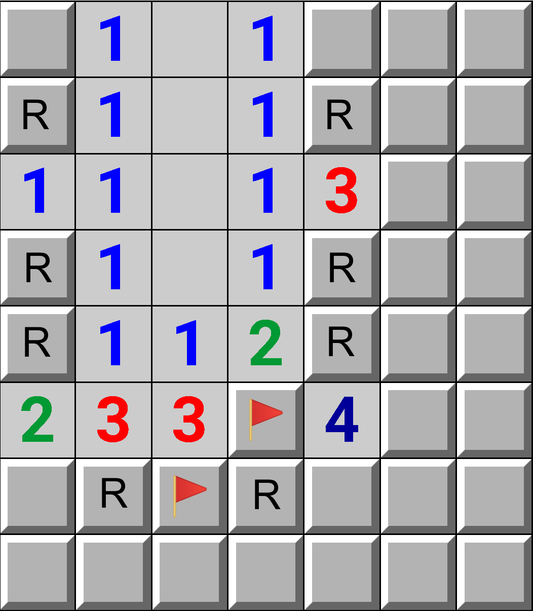
An example:
The [green/red] squares are the squares where running local deductions determined they [didn't/did] have mines. Notice local deductions have failed to find all possible deducible squares (there's a 2-1 pattern on the top row).
Before running local deductions, there is 1 component with 28 squares. The backtracking would have taken \(\sim 28\cdot2^{28} = 7,516,192,768\) operations. After running local deductions, there's 1 component with 9 non-deduced squares (\(9\cdot2^9 = 4,608\)).
Although this optimization seems like it would help a lot, there are many cases where this optimization doesn't help out much (for example, consider if there are no deducible squares).
Further Splitting of Components
Let's define the problem: You are given a single component of \(n\) squares (labeled 1, 2, ..., n). Find:
- \(\#configs[]\) defined as: \(\#configs[i]\) = the number of mine configurations with \(i\) mines, (\(0 \leq i \leq M\))
- \(\#configsWithJMine[][]\) defined as: \(\#configsWithJMine[i][j]\) = the number of mine configurations which have \(i\) mines, and square \(j\) is a mine, (\(0 \leq i \leq M, 1 \leq j \leq n\))
This of course can be solved with recursive backtracking in \(\mathcal{O}(n\cdot2^n)\). Let's try to solve this problem faster as it is usually the bottleneck of the entire mine probability calculation (every other step runs in polynomial time).
Consider the following board.
Imagine if we somehow "removed" the un-discovered square next to the 1.
Then, the board would contain 2 components.
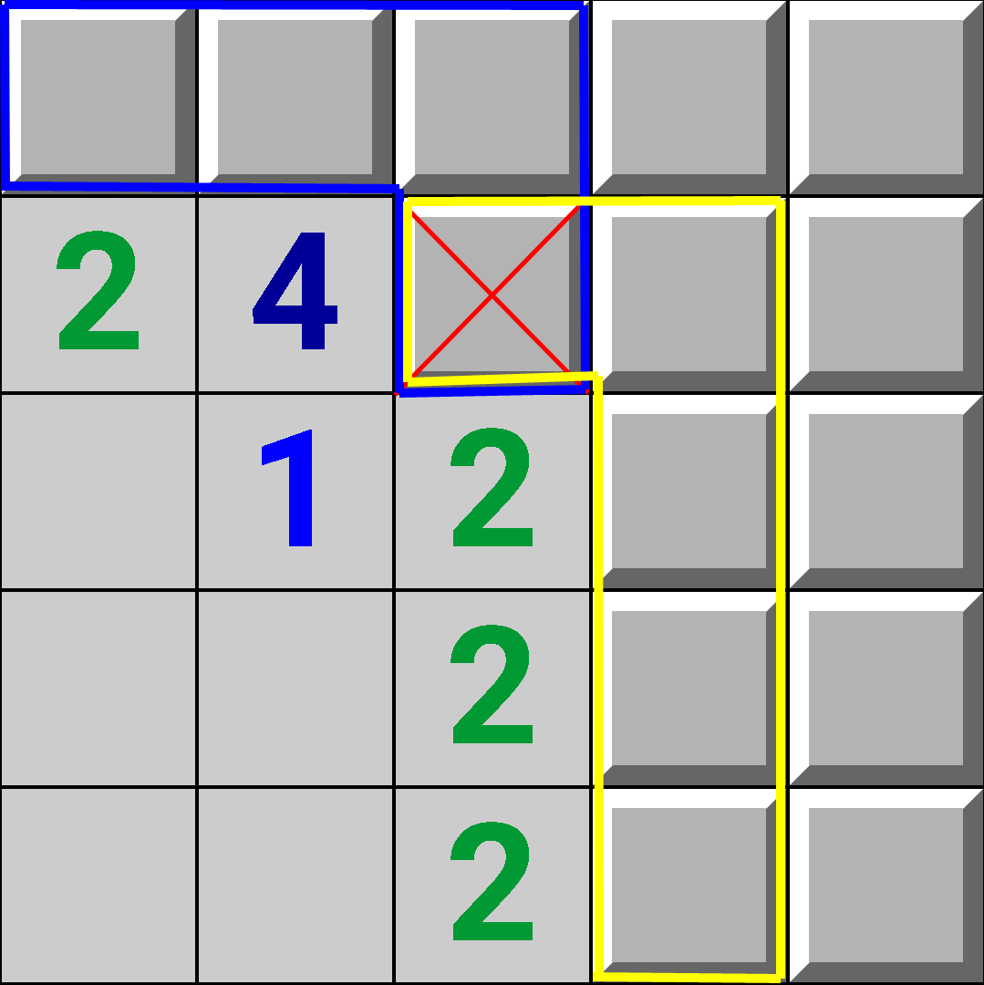
Now, what if we ran the backtracking independently on both the blue and yellow components, and then somehow combined the results? In this way, we can take a single component, and split it further into \(\geq 2\) smaller components.
But why limit ourselves to splitting a single component once? Notice, we have to solve the exact same problem for both the blue and yellow components. Thus, why solve it with backtracking, when we can again use the same trick of "removing" squares? This leads to the following recursive algorithm.
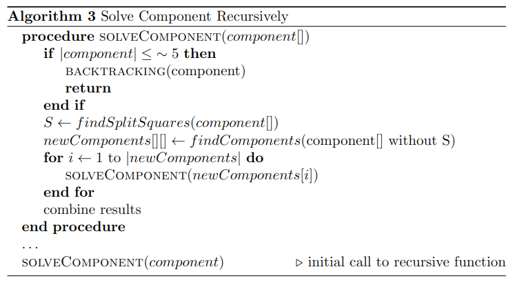
Here, the "split" squares are the squares which we remove to split up the original component. Before diving into the reasons why this algorithm is still exponential, I'll explain the following parts:
- the \(findSplitSquares\) function
- combining results
Finding Split Squares
First, we don't have to limit ourselves to removing just 1 square to split components. Although, assuming we remove \(k\) squares, it turns out the combine step will take \(\mathcal{O}(2^k)\) time. So in my implementation, I arbitrarily chose 6 as an upper bound on the number of split squares.
Finding split squares requires representing the minesweeper board as a graph:
- squares are nodes
- 2 squares share an edge if there exists a number next to both squares
For example this board,
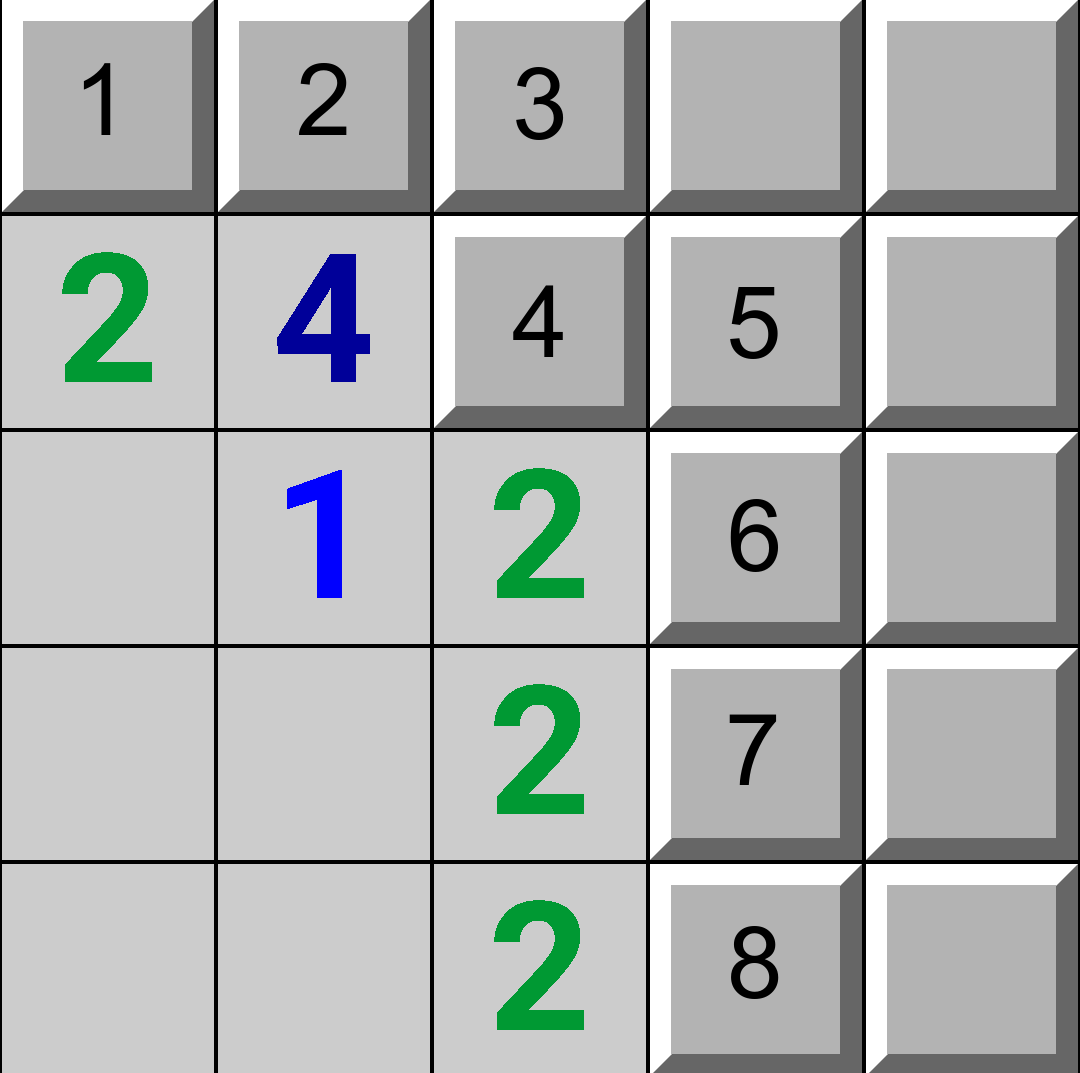 ,
produces the following graph:
,
produces the following graph:
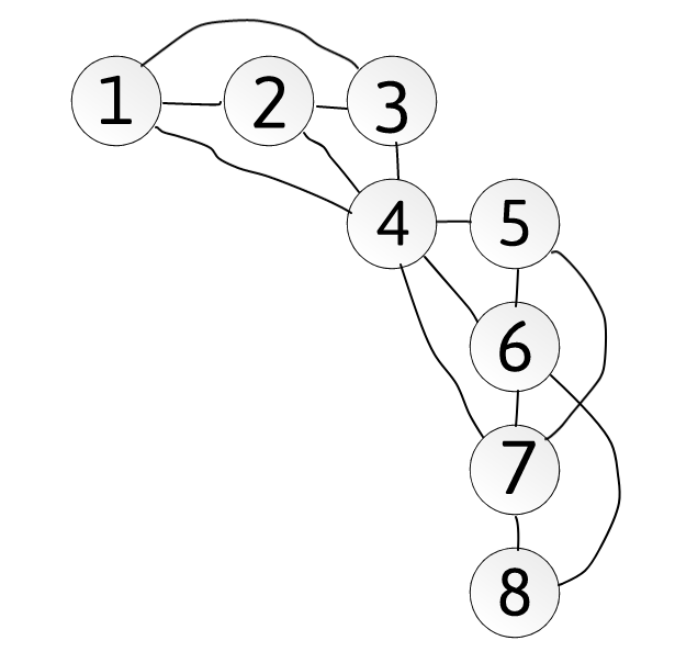
Notice that if node 4 is removed, then the graph would split
into 2 connected components. Thus node 4 is an
articulation node.
The first attempt would be to choose \(\leq\) 6 articulation nodes
from the graph to remove. Although this approach would
fail on grids such as:
 whose graphs have no articulation nodes. So let's find a more
generalized solution.
whose graphs have no articulation nodes. So let's find a more
generalized solution.
Ideally, we would want to remove \(\leq\) 6 nodes such that the size of the largest component is minimized. Unfortunately, the generalized problem of finding k nodes to remove to minimize the size of the largest remaining component is NP-complete. But this isn't as relevant as you'd think. There are at least 2 options:
- employ an approximation algorithm such as the 2-exchange method
- employ a brute force approach similar to this comment. Brute force here is okay since we're only removing \(\leq\) 6 nodes (thus is exponential in 6).
Combining Results
Recall the problem: you are given a single component of \(n\) squares (labeled 1, 2, ..., n). Find:
- \(\#configs[]\) defined as: \(\#configs[i]\) = the number of mine configurations with \(i\) mines, (\(0 \leq i \leq M\))
- \(\#configsWithJMine[][]\) defined as: \(\#configsWithJMine[i][j]\) = the number of mine configurations which have \(i\) mines, and square \(j\) is a mine, (\(0 \leq i \leq M, 1 \leq j \leq n\))
I'll only explain how to calculate \(\#configs[]\) as \(\#configsWithJMine[][]\) is calculated very similarly.
To understand this section, it'll help to know about dynamic programming with bitmasks. Consider this example board again:
Our goal is to calculate some sub-result (not necessarily \(\#configs[]\)) for both the blue and yellow components, and then calculate the same sub-result for the original component. Also, we have to be able to calculate \(\#configs[]\) from this sub-result.
The sub-result is an array \(dp[][]\) defined as: \(dp[mask][i]\) = the number of mine configurations with \(i\) mines under the restriction that if and only if the \(j\)-th bit in \(mask\) is 1, then there is a mine in the \(j\)-th removed square.
Since the above example has only 1 removed square we consider 2 cases:
- the removed square is a mine \(\left(mask = 1\right)\)
- the removed square is not a mine \(\left(mask = 0\right)\)
If the removed square is a mine, we have \[dpOriginal[1][i] = \sum \limits_{j=0}^{i+1} dpBlue[1][j] \cdot dpYellow[1][i+1-j]\] where:
- \(dpOriginal[][]\) is the \(dp[][]\) array corresponding to the original component
- \(dpBlue[][]\) is the \(dp[][]\) array corresponding to the blue component
- \(dpYellow[][]\) is the \(dp[][]\) array corresponding to the yellow component
Notice the upper bound on the sum is curiously \(\left(i+1\right)\). Both the blue and yellow components have a mine in the removed square. Thus we end up double counting this mine. The \(\left(i+1\right)\) upper limit cancels out with the double counting to get the correct result.
If the removed square is not a mine, we have \[dpOriginal[0][i] = \sum \limits_{j=0}^i dpBlue[0][j] \cdot dpYellow[0][i-j].\] Assuming there are \(k\) removed squares \(\left(k \leq 6\right)\), we have \[\#configs[i] = \sum \limits_{mask=0}^{2^k-1} dp[mask][i].\] Here, there are \(2^k\) masks as there are \(2^k\) possible ways to place mines among the \(k\) removed squares.
Finally, the original recursive call has 0 removed squares, so \(2^0 = 1\), there's 1 possible mask \(\left(mask = 0\right)\), and the \(\#configs\) array is stored in \(dp[0].\)
In this example, the original component was split into 2 sub-components, but in general, the original component can be split into \(k\) sub-components. It is possible to generalize this knapsack-like dynamic programming to work for \(k\) sub-components.
There is a tricky case where a clue is surrounded by only "removed" squares. Make sure to skip the masks which have the incorrect number of mines for these clues.
Discussion on this Recursive Algorithm
Why is this algorithm still exponential? Consider the case where all of the \(\binom{n}{\leq 6}\) subsets of nodes to remove don't decrease the size of the component (there's still 1 component after removing nodes). In this case, we're forced to solve the problem with normal recursive backtracking in \(\mathcal{O}(n\cdot2^n)\). Although in practice, this case is super rare.
Where does the speedup come from with this recursive approach? For recursive backtracking, even with the best possible pruning, you'll still hit the base case once for every mine configuration. Thus, recursive backtracking has a lower bound of \(\Omega\left(\text{number of mine configurations}\right)\). This new recursive approach doesn't have the same lower bound, and thus potentially can be faster (and is faster in practice).
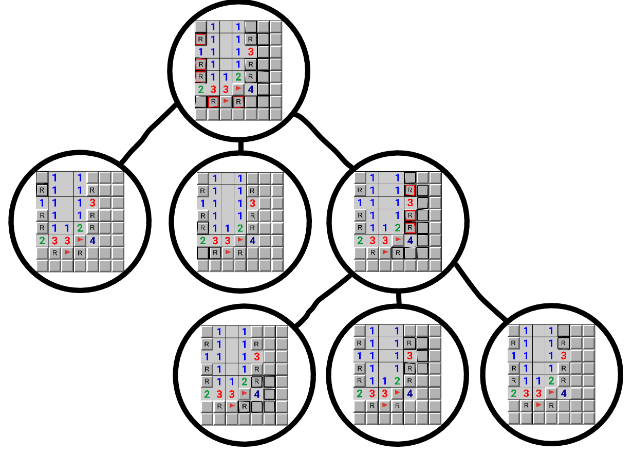
Finally, here's a picture of the recursion tree for the board:
 .
Here, the squares marked with an "R" are articulation nodes in
the corresponding graph. If you remove any of the "R" squares,
the board will split into 2 components (not considering the
flagged squares).
.
Here, the squares marked with an "R" are articulation nodes in
the corresponding graph. If you remove any of the "R" squares,
the board will split into 2 components (not considering the
flagged squares).
 .
.
- Each node in this tree represents a single recursive call
- Squares surrounded in black are in the sub-component in the current recursive call
- Squares surrounded in both black and red are the "removed" squares which are used to further split the current component
- Leaf node components are solved with recursive backtracking